differences between two ways of calculating the mean
specifying the response variable and offset in a Tweedie regression model depending on the quantity of interest
log-likelihood and the corresponding score function for a Tweedie model with weights
why one way of specifying offsets in poisson GLMs with the identity link does not extend to Tweedie GLMs
In this article, the words duration, offset, exposure, and weight are used interchangeably.
Introduction
Data coming from fields like ecology, insurance, epidemiology – such as number of new cases of a disease in multiple cities with very different population sizes, number of claims and total claim amounts from insurance policies with different durations, etc. – need to have the varying exposures accounted for as offsets while building models. These might look something like the following simulated dataset with an exposure variable (w) and a response variable (y):
library(tidyverse)
── Attaching core tidyverse packages ──────────────────────── tidyverse 2.0.0 ──
✔ dplyr     1.1.2     ✔ readr     2.1.4
✔ forcats   1.0.0     ✔ stringr   1.5.0
✔ ggplot2   3.4.2     ✔ tibble    3.2.1
✔ lubridate 1.9.2     ✔ tidyr     1.3.0
✔ purrr     1.0.1
── Conflicts ────────────────────────────────────────── tidyverse_conflicts() ──
✖ dplyr::filter() masks stats::filter()
✖ dplyr::lag()    masks stats::lag()
ℹ Use the conflicted package (<http://conflicted.r-lib.org/>) to force all conflicts to become errors
n <-1e6# tweedie distribution parametersp <-1.3# variance powermu <-200# meanphi <-350# dispersion, so variance = phi * mu ^ pset.seed(45)sim_data <-tibble(w =runif(n, min =0.5, max =3),y = tweedie::rtweedie(n = n, mu = mu, phi = phi / w, power = p))# summary(sim_data)sim_data %>%slice_head(n =3)
# A tibble: 3 × 2
      w     y
  <dbl> <dbl>
1  2.08     0
2  1.29     0
3  1.10     0
For readability, let’s pretend that this response variable is the individual claim amounts for an insurance company with a client base of 1 million customers. Additionally, for each individual the duration of how long they’ve been insured is also recorded. So the first customer has been insured for about 2 years and 1 month, and has not filed a claim at all. The third customer has been insured for a little over a year and has also not filed any claims.
Ratio of means or mean of ratios?
The quantity of interest from such datasets may be the mean per unit exposure – expected claim amount per individual per year, expected number of new cases of a disease per year per 100,000 people, etc. There are two separate quantities that can be calculated as expected values – the ratio of the means of amount and duration variables, or the mean of the individual ratios. The differences between these two quantities is explained pretty well in this stackexchange thread.
The ratio estimator estimates the first quantity \(R = \sum_i{y_i} / \sum_i{w_i}\). This answers the following question: given a population (or a group of individuals) who were followed-up / observed for a given amount of time, and generated a total amount of claims, how much of the total claim amount can be attributed per person per unit exposure?
The weighted sample mean of the individual ratios estimates the second quantity \(\mathbb{E} = \sum_i{w_i y_i} / \sum_i{w_i}\). This answers the question: given each individual’s claim amount and exposure, what was the average individual’s claim amount per unit exposure?
In the latter case, the link between claim amount and duration at the individual level is preserved, whereas for the former, the numerator and denominators are totals at the population level.
If everyone had exactly the same weight \(w_i\) of 1 year, the denominator would sum to the sample size of 1 million for the data above, and both the estimates would be the same. If the weights were different, then the two results would differ.
In epidemiology, the ratio estimator is used for incidence rate calculations. On the other hand, the insurance papers on Tweedie models mentioned at the bottom of this post all seem to use the weighted mean approach.
For the simulated data above, the two estimates are quite different:
sum(sim_data$y) /sum(sim_data$w)
[1] 114.5185
weighted.mean(sim_data$y, w = sim_data$w)
[1] 200.4661
In this case, the second estimate matches the true mean value chosen for the simulation, which makes sense given that the data are simulated from a Tweedie model with varying exposures (\(Y_i \sim \text{Tweedie}(\mu_i, \phi / w_i, p)\)) but with the mean-variance relationship preserved under unit exposure. This is described in part A of the supplement to the Yang et al 2016 paper.
However, both the numbers are right, as they answer different questions.
Building a regression model
This formula is easy enough to apply if there are no predictors, but a regression model is needed to estimate these quantities when there are predictors in the data.
There are two ways of specifying the model. The first method corresponds to passing the claim amounts unmodified, and passing the exposures as weights:
# weighted mean estimatorsummary(glm(y ~1, weights = w, data = sim_data,family = statmod::tweedie(var.power =1.3, link.power =1)))
Call:
glm(formula = y ~ 1, family = statmod::tweedie(var.power = 1.3,
    link.power = 1), data = sim_data, weights = w)

Coefficients:
            Estimate Std. Error t value Pr(>|t|)
(Intercept) 200.4661     0.4431   452.4   <2e-16 ***
---
Signif. codes:  0 '***' 0.001 '**' 0.01 '*' 0.05 '.' 0.1 ' ' 1

(Dispersion parameter for Tweedie family taken to be 349.4572)

    Null deviance: 240499666  on 999999  degrees of freedom
Residual deviance: 240499666  on 999999  degrees of freedom
AIC: NA

Number of Fisher Scoring iterations: 3
The estimated intercept and dispersion correspond to the same parameters (\(\mu = 200\), \(\phi = 350\)) picked for the simulation. This estimate also coincides with the weighted mean estimate. link.power = 1 indicates that the identity link function is used, and var.power = 1.3 or \(p = 1.3\) is assumed to be known here. Usually the profile likelihood approach is used to pick the best value on the interval \(p \in (1, 2)\) for data with exact zeroes.
Once \(p\) is chosen, \(\mu\) can be estimated independently of \(\phi\), and finally dispersion \(\phi\) can be estimated using an optimization algorithm, or one of the estimators described in section 6.8 of the Dunn and Smyth book. The glm function in R uses the Pearson estimator:
The second method rescales the response variable with the weights, and passes exposures as weights to the model:
# ratio estimatorsummary(glm(y / w ~1, weights = w, data = sim_data,family = statmod::tweedie(var.power =1.3, link.power =1)))
Call:
glm(formula = y/w ~ 1, family = statmod::tweedie(var.power = 1.3,
    link.power = 1), data = sim_data, weights = w)

Coefficients:
            Estimate Std. Error t value Pr(>|t|)
(Intercept) 114.5185     0.3655   313.3   <2e-16 ***
---
Signif. codes:  0 '***' 0.001 '**' 0.01 '*' 0.05 '.' 0.1 ' ' 1

(Dispersion parameter for Tweedie family taken to be 492.3754)

    Null deviance: 177557174  on 999999  degrees of freedom
Residual deviance: 177557174  on 999999  degrees of freedom
AIC: NA

Number of Fisher Scoring iterations: 3
This estimate corresponds to the same output as the ratio estimator from the previous section. The estimate of dispersion \(\phi\) is different from the true value of 350, which makes sense as dispersion is a function of the estimated value of the mean \(\mu\).
What does the math look like behind these two models?
To fit a Tweedie model to the data with weights to calculate the two different values in the previous section, the following log-likelihood function – taken from the Yang et al paper – can be maximized.
For this simulated dataset, \(w_i\) and \(y_i\) vary for each individual, but there are no predictors so an identity link function can be used 1, the overall mean is of interest so the \(\mu_i\) term can be collapsed into a single \(\mu\) parameter to be optimized, and the log a(...) term can be ignored as it’s not a function of \(\mu\). Since the regression equation for an intercept only term is \(\mu_i = \beta_0\), we can replace the \(\mu\) with \(\beta_0\).
1 which should be avoided if the model will be used for out-of-sample prediction to avoid predicting values below 0
This makes it easy to compute the closed form solution, which is calculated by differentiating this function to produce the score function, and setting it to 0.
A method that works for Poisson but not for Tweedie
What initially led me down this rabbit hole was finding this stackexchange post for specifying the offset with identity link in a poisson model, and naively (and incorrectly) fitting the Tweedie glm like this
summary(glm(y ~ w -1, data = sim_data,family = statmod::tweedie(var.power =1.3, link.power =1)))
Call:
glm(formula = y ~ w - 1, family = statmod::tweedie(var.power = 1.3,
    link.power = 1), data = sim_data)

Coefficients:
  Estimate Std. Error t value Pr(>|t|)
w 121.7328     0.4064   299.6   <2e-16 ***
---
Signif. codes:  0 '***' 0.001 '**' 0.01 '*' 0.05 '.' 0.1 ' ' 1

(Dispersion parameter for Tweedie family taken to be 465.8885)

    Null deviance:       NaN  on 1000000  degrees of freedom
Residual deviance: 158130565  on  999999  degrees of freedom
AIC: NA

Number of Fisher Scoring iterations: 3
and trying to figure out why this didn’t coincide with the ratio estimate of 114.5185, which is the case for the poisson models
# ratio estimatorsum(sim_data$y) /sum(sim_data$w)
[1] 114.5185
# generates warnings because we're passing a non-discrete response# point estimates are the same thoughunname(coef(suppressWarnings(glm(y ~ w -1, family =poisson(link ="identity"), data = sim_data))))
[1] 114.5185
unname(coef(suppressWarnings(glm(y / w ~1, weights = w, family =poisson(link ="identity"), data = sim_data))))
[1] 114.5185
This happens because substituting \(\mu_i = w_i \beta_0\) instead of \(\mu_i = \beta_0\) in the log-likelihood function
The constant \(\phi\) and \(\beta_0^{-p}\) terms can be dropped from the equation, and the \(w_i\) outside the bracket are all 1 because no weights are passed to the glm call, so the following equation is solved
This shows where the logical error happens, as well as how the correct estimate can be obtained, i.e., by passing weights = w ^ (p - 1) to the glm call, so that the \(w_i^{1-p}\) term cancels out
summary(glm(y ~ w -1, weights =I(w^(1.3-1)), data = sim_data,family = statmod::tweedie(var.power =1.3, link.power =1)))
Call:
glm(formula = y ~ w - 1, family = statmod::tweedie(var.power = 1.3,
    link.power = 1), data = sim_data, weights = I(w^(1.3 - 1)))

Coefficients:
  Estimate Std. Error t value Pr(>|t|)
w 114.5185     0.3655   313.3   <2e-16 ***
---
Signif. codes:  0 '***' 0.001 '**' 0.01 '*' 0.05 '.' 0.1 ' ' 1

(Dispersion parameter for Tweedie family taken to be 492.3754)

    Null deviance:       NaN  on 1000000  degrees of freedom
Residual deviance: 177557174  on  999999  degrees of freedom
AIC: NA

Number of Fisher Scoring iterations: 3
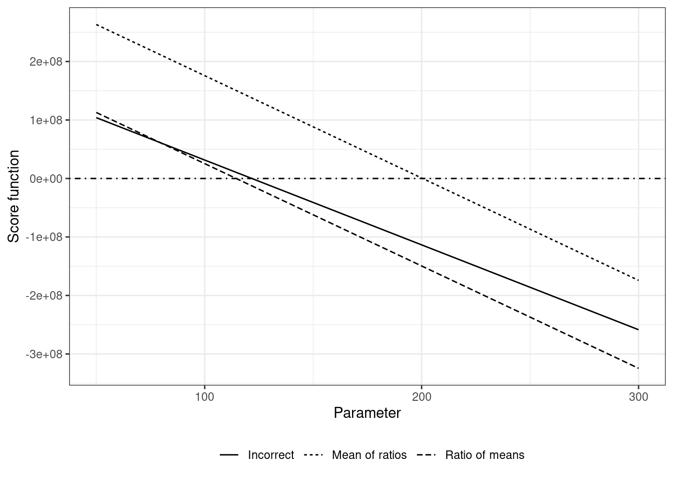
Now the point estimates, standard errors, and dispersion parameters correspond to the model where the ratio estimator is correctly specified.
Here’s the code and the plot of the score equations for the different models:
---title: "Specifying an offset in a Tweedie model with identity link"date: "2023-07-30"categories: [R, Tweedie, Offset]code-fold: falsereference-location: marginimage: "tweedie-image.png"---This post explores several things:- differences between two ways of calculating the mean- specifying the response variable and offset in a Tweedie regression model depending on the quantity of interest- log-likelihood and the corresponding score function for a Tweedie model with weights- why one way of specifying offsets in poisson GLMs with the identity link does not extend to Tweedie GLMsIn this article, the words duration, offset, exposure, and weight are used interchangeably.## IntroductionData coming from fields like ecology, insurance, epidemiology -- such as number of new cases of a disease in multiple cities with very different population sizes, number of claims and total claim amounts from insurance policies with different durations, etc. -- need to have the varying exposures accounted for as offsets while building models. These might look something like the following simulated dataset with an exposure variable (w) and a response variable (y):```{r}library(tidyverse)n <-1e6# tweedie distribution parametersp <-1.3# variance powermu <-200# meanphi <-350# dispersion, so variance = phi * mu ^ pset.seed(45)sim_data <-tibble(w =runif(n, min =0.5, max =3),y = tweedie::rtweedie(n = n, mu = mu, phi = phi / w, power = p))# summary(sim_data)sim_data %>%slice_head(n =3)```For readability, let's pretend that this response variable is the individual claim amounts for an insurance company with a client base of 1 million customers. Additionally, for each individual the duration of how long they've been insured is also recorded. So the first customer has been insured for about 2 years and 1 month, and has not filed a claim at all. The third customer has been insured for a little over a year and has also not filed any claims.## Ratio of means or mean of ratios?The quantity of interest from such datasets may be the mean per unit exposure -- expected claim amount per individual per year, expected number of new cases of a disease per year per 100,000 people, etc. There are two separate quantities that can be calculated as expected values -- the ratio of the means of amount and duration variables, or the mean of the individual ratios. The differences between these two quantities is explained pretty well in [this stackexchange thread](https://stats.stackexchange.com/a/105715).The [ratio estimator](https://en.wikipedia.org/wiki/Ratio_estimator) estimates the first quantity $R = \sum_i{y_i} / \sum_i{w_i}$. This answers the following question: given a population (or a group of individuals) who were followed-up / observed for a given amount of time, and generated a total amount of claims, how much of the total claim amount can be attributed per person per unit exposure?The [weighted sample mean](https://en.wikipedia.org/wiki/Weighted_arithmetic_mean) of the individual ratios estimates the second quantity $\mathbb{E} = \sum_i{w_i y_i} / \sum_i{w_i}$. This answers the question: given each individual's claim amount and exposure, what was the average individual's claim amount per unit exposure?In the latter case, the link between claim amount and duration at the individual level is preserved, whereas for the former, the numerator and denominators are totals at the population level.If everyone had exactly the same weight $w_i$ of 1 year, the denominator would sum to the sample size of 1 million for the data above, and both the estimates would be the same. If the weights were different, then the two results would differ.In epidemiology, the ratio estimator is used for *incidence rate* calculations. On the other hand, the insurance papers on Tweedie models mentioned at the bottom of this post all seem to use the weighted mean approach.For the simulated data above, the two estimates are quite different:```{r}sum(sim_data$y) /sum(sim_data$w)``````{r}weighted.mean(sim_data$y, w = sim_data$w)```In this case, the second estimate matches the true mean value chosen for the simulation, which makes sense given that the data are simulated from a Tweedie model with varying exposures ($Y_i \sim \text{Tweedie}(\mu_i, \phi / w_i, p)$) but with the mean-variance relationship preserved under unit exposure. This is described in part A of the supplement to the Yang et al 2016 paper.However, both the numbers are right, as they answer different questions.## Building a regression modelThis formula is easy enough to apply if there are no predictors, but a regression model is needed to estimate these quantities when there are predictors in the data.There are two ways of specifying the model. The first method corresponds to passing the claim amounts unmodified, and passing the exposures as weights:```{r}# weighted mean estimatorsummary(glm(y ~1, weights = w, data = sim_data,family = statmod::tweedie(var.power =1.3, link.power =1)))```The estimated intercept and dispersion correspond to the same parameters ($\mu = 200$, $\phi = 350$) picked for the simulation. This estimate also coincides with the weighted mean estimate. `link.power = 1` indicates that the identity link function is used, and `var.power = 1.3` or $p = 1.3$ is assumed to be known here. Usually the profile likelihood approach is used to pick the best value on the interval $p \in (1, 2)$ for data with exact zeroes.Once $p$ is chosen, $\mu$ can be estimated independently of $\phi$, and finally dispersion $\phi$ can be estimated using an optimization algorithm, or one of the estimators described in section 6.8 of the Dunn and Smyth book. The glm function in R uses the *Pearson estimator*:$$\phi = \frac{1}{N-p'} \sum_{i=1}^{N} \frac{w_i (y_i - \hat\mu_i) ^ 2}{\hat\mu_i^p}$$where $p'$ is the number of parameters in the model and $\text{Var}(\mu_i) = \mu_i^p$ is the variance function.```{r}# pearson estimate of dispersion(sum((sim_data$w * ((sim_data$y -200.4661)^2)) / (200.4661^1.3))) / (n -1)```The second method rescales the response variable with the weights, and passes exposures as weights to the model:```{r}# ratio estimatorsummary(glm(y / w ~1, weights = w, data = sim_data,family = statmod::tweedie(var.power =1.3, link.power =1)))```This estimate corresponds to the same output as the ratio estimator from the previous section. The estimate of dispersion $\phi$ is different from the true value of 350, which makes sense as dispersion is a function of the estimated value of the mean $\mu$.## What does the math look like behind these two models?To fit a Tweedie model to the data with weights to calculate the two different values in the previous section, the following log-likelihood function -- taken from the Yang et al paper -- can be maximized.$$l(\mu, \phi, p | \{y, x, w\}_{i=1}^n) = \sum_{i = 1}^{n}{ \frac{w_i}{\phi}} \Bigg(y_i \frac{\mu_i^{1-p}}{1-p} - \frac{\mu_i^{2-p}}{2-p} \Bigg) + log\ a(y_i, \phi / w_i, p)$$For this simulated dataset, $w_i$ and $y_i$ vary for each individual, but there are no predictors so an identity link function can be used [^1], the overall mean is of interest so the $\mu_i$ term can be collapsed into a single $\mu$ parameter to be optimized, and the `log a(...)` term can be ignored as it's not a function of $\mu$. Since the regression equation for an intercept only term is $\mu_i = \beta_0$, we can replace the $\mu$ with $\beta_0$.[^1]: which should be avoided if the model will be used for out-of-sample prediction to avoid predicting values below 0This makes it easy to compute the closed form solution, which is calculated by differentiating this function to produce the score function, and setting it to 0.$$\frac{\partial l}{\partial \beta} = \sum_{i = 1}^{n}{ \frac{w_i}{\phi}} (y_i \beta_0^{-p} - \beta_0^{1-p}) = 0$$$\phi$ and $\beta_0^{-p}$ are non-zero constants, so can be pulled out of the summation and absorbed into the zero on the right-hand side to give$$\sum_{i = 1}^{n}{ w_i (y_i - \beta_0) } = 0$$For `glm(y ~ 1, weights = w, ...)`, this equals$$\sum_{i = 1}^{n} w_i y_i - \beta_0 \sum_{i = 1}^{n} w_i = 0 \\\Rightarrow \beta_0 = \frac{\sum_{i = 1}^{n} {w_i y_i}}{\sum_{i = 1}^{n} w_i}$$and for `glm(y / w ~ 1, weights = w, ...)`, this equals$$\sum_{i = 1}^{n} w_i \frac{y_i}{w_i} - \beta_0 \sum_{i = 1}^{n} w_i = 0 \\\Rightarrow \beta_0 = \frac{\sum_{i = 1}^{n} {y_i}}{\sum_{i = 1}^{n} w_i}$$## A method that works for Poisson but not for TweedieWhat initially led me down this rabbit hole was finding [this stackexchange post](https://stats.stackexchange.com/questions/275893/offset-in-poisson-regression-when-using-an-identity-link-function) for specifying the offset with identity link in a poisson model, and naively (and incorrectly) fitting the Tweedie glm like this```{r}summary(glm(y ~ w -1, data = sim_data,family = statmod::tweedie(var.power =1.3, link.power =1)))```and trying to figure out why this didn't coincide with the ratio estimate of 114.5185, which is the case for the poisson models```{r, warning=FALSE}# ratio estimatorsum(sim_data$y) /sum(sim_data$w)# generates warnings because we're passing a non-discrete response# point estimates are the same thoughunname(coef(suppressWarnings(glm(y ~ w -1, family =poisson(link ="identity"), data = sim_data))))unname(coef(suppressWarnings(glm(y / w ~1, weights = w, family =poisson(link ="identity"), data = sim_data))))```This happens because substituting $\mu_i = w_i \beta_0$ instead of $\mu_i = \beta_0$ in the log-likelihood function$$l(\beta_0, \phi, p | \{y, x, w\}_{i=1}^n) = \sum_{i = 1}^{n}{ \frac{w_i}{\phi}} \Bigg(y_i \frac{(w_i \beta_0)^{1-p}}{1-p} - \frac{(w_i\beta_0)^{2-p}}{2-p} \Bigg) + log\ a(y_i, \phi / w_i, p)$$leads to the following score function$$\frac{\partial l}{\partial \beta} = \sum_{i = 1}^{n} \frac{w_i}{\phi} (y_i w_i^{1-p} \beta_0^{-p} - w_i^{2-p} \beta_0^{1-p}) = 0$$The constant $\phi$ and $\beta_0^{-p}$ terms can be dropped from the equation, and the $w_i$ outside the bracket are all 1 because no weights are passed to the glm call, so the following equation is solved$$\sum_{i = 1}^{n} y_i w_i^{1-p} - w_i^{2-p} \beta_0 = 0$$which can be simplified by pulling $w_i^{1-p}$ as a common term$$\sum_{i = 1}^{n} w_i^{1-p} (y_i - w_i \beta_0) = 0$$This shows where the logical error happens, as well as how the correct estimate can be obtained, i.e., by passing `weights = w ^ (p - 1)` to the glm call, so that the $w_i^{1-p}$ term cancels out```{r}summary(glm(y ~ w -1, weights =I(w^(1.3-1)), data = sim_data,family = statmod::tweedie(var.power =1.3, link.power =1)))```Now the point estimates, standard errors, and dispersion parameters correspond to the model where the ratio estimator is correctly specified.Here's the code and the plot of the score equations for the different models:```{r}#| code-fold: trueparameter_grid <-seq(50, 300, 5)estimating_equation_curves <-tibble(parameter = parameter_grid,`Mean of ratios`=map_dbl(.x = parameter_grid, .f =~ { sim_data %>%mutate(s = w * (y - .x)) %>%pull(s) %>%sum() }),`Ratio of means`=map_dbl(.x = parameter_grid, .f =~ { sim_data %>%summarize(across(.cols =c(w, y), .fns = sum)) %>%mutate(s = y - (.x * w)) %>%pull(s) }),Incorrect =map_dbl(.x = parameter_grid, .f =~ { sim_data %>%mutate(s = (w ^ (1-1.3)) * (y - w * .x)) %>%pull(s) %>%sum() }))estimating_equation_curves %>%pivot_longer(-parameter) %>%ggplot(aes(x = parameter, y = value, linetype = name)) +geom_line() +geom_hline(yintercept =0, linetype ="dotdash") +# geom_vline(xintercept = 114.5185, linetype = 2) +# geom_vline(xintercept = 121.7328, linetype = 1) +# geom_vline(xintercept = 200, linetype = 11) +theme_bw() +ylab("Score function") +xlab("Parameter") +theme(legend.position ="bottom", legend.title =element_blank())```## References- Yang et al 2016 paper and supplement ([link](https://www.tandfonline.com/doi/full/10.1080/07350015.2016.1200981))- Delong et al 2021 paper ([link](https://link.springer.com/article/10.1007/s13385-021-00264-3))- Chapter 12 on Tweedie models from the Dunn and Smyth book on GLMsOthers- Zhang 2013 ([link](https://link.springer.com/article/10.1007/s11222-012-9343-7))- Stan code for Tweedie - <https://discourse.mc-stan.org/t/tweedie-likelihood-compound-poisson-gamma-in-stan/14636> - [this gist](https://gist.github.com/MatsuuraKentaro/952b3301686c10adcb13){.uri}